Lets Make a Map: Baltimore Edition

I recently came across an excellent tutorial written by Mike Bostock for creating a map from scratch using D3 and TopoJSON. I thought that I would use it as a starting point to create a map of Baltimore using data from the U.S. Census Bureau.

Get the Data

We will be using data from the U.S. Census Bureau to create a map of Baltimore. The U.S. Census Bureau calls this data “TIGER Products,” an acronym for Topologically Integrated Geographic Encoding and Referencing. This data includes topological overlays for things such as congressional districts, census blocks, and state and county boundaries as well as features such as roads, rail lines and water features. Many of these products are available at different resolutions. The Census Bureau provides a immense amount of geographic data but wading through it can be challenging.

We are particularly interested in the TIGER/Line Shapefiles product. This data product is suitable for use with GIS and contains the most detail. We want the Maryland places, Baltimore City all lines, and Baltimore City water area layers, which can be downloaded from the TIGER/Line Shapefiles web interface and are named:

• tl_2013_24_place.zip
• tl_2013_24510_edges.zip
• tl_2013_24510_areawater.zip

TIGER/Line Shapefiles follow a naming convention. For these archives, “2013” represents the year of the data set, “24” is the Maryland state code, and “24510” is the Maryland state code concatenated with “510”, the code for Baltimore city. Unzip each of these archives.

Install the Tools

We will be using the same tools in the original article. To recap:

• Install the Geospacial Data Abstraction Library (GDAL) using Homebrew if you on a Mac by entering brew install gdal on the command line.
• Install Node.js to acquire the reference TopoJSON implementation. You can do this by entering brew install node and then npm install -g topojson on the command line.

Convert the Data

First, we will use the ogr2ogr binary installed with GDAL to convert the Shapefiles we downloaded into GeoJSON, filtering out only the features that we need. The Shapefiles are stored in a database and features can be extracted using SQL queries. On the command line, move into the tl_2013_24_place/ directory and enter:

gr2ogr -f GeoJSON -sql "SELECT NAME as FULLNAME from tl_2013_24_place WHERE NAME in ('Baltimore')" baltimore.json tl_2013_24_place.shp

This command takes the Maryland places layer and uses an SQL query to select the features where the NAME column value is Baltimore and convert them to the GeoJSON file baltimore.json. In addition, it renames the NAME column to FULLNAME which we will need for a later step.

Next, move into the tl_2013_24510_edges/ directory and enter:

ogr2ogr -f GeoJSON baltimore_edges.json -where "MTFCC IN ('H3010', 'P0002', 'P0003', 'S1100')" tl_2013_24510_edges.shp

This filters the Baltimore City edges layer for features with the MAF/TIGER Feature Class Codes (MTFCC) matching those for coastlines (P0002 and P0003), streams and rivers (H3010), and major roads (S1100) and converts them to the GeoJSON file baltimore_edges.json. The U.S. Census Bureau has a PDF containing a description of each MTFCC.

Lastly, move into the tl_2013_24510_areawater/ directory and convert the last Shapefile to GeoJSON by entering:

ogr2ogr -f GeoJSON baltimore_water.json tl_2013_24510_areawater.shp

Now that we’ve made our baltimore.json, baltimore_edges.json, and baltimore_water.json GeoJSON files it would be a good time to move them to the same directory. We will convert them to TopoJSON format by entering the following command on the command line:

topojson -o balt.json --id-property=TLID --properties name=FULLNAME,code=MTFCC baltimore.json baltimore_edges.json baltimore_water.json

This command combines the GeoJSON files into one TopoJSON file named balt.json with only the FULLNAME and MTFCC properties. We can see the result of the topojson command by looking at the structure of balt.json:

{
  "type": "Topology",
  "objects": {
    "baltimore": {
      "type": "GeometryCollection",
      "geometries": [
        {
          "type":"Polygon",
          "properties": { "name":"Baltimore" },
          ...
         },
         ...
       ]
    },
    "baltimore_edges": {
      "type": "GeometryCollection",
      "geometries": [
        {
          "type": "LineString",
          "properties": { "name":"Western Run", "code":"H3010" },
          "id": 206404412
          ...
        },
        ...
      ]
    },
    ...
  }
}

There are a few things to take note of here:

• The names of each GeoJSON file have become keys underneath objects in the TopoJSON file.
• The features in each GeoJSON file have become objects in the corresponding geometries lists in the TopoJSON file.
• The --id-property=TLID flag in the topojson command mapped each feature’s TLID field to the id key.
• The --properties name=FULLNAME,code=MTFCC flag for the topojson command mapped FULLNAME to name and MTFCC to code under properties in the TopoJSON file.

Write Some HTML

Our starting index.html file looks like the following:

<!DOCTYPE html>
<meta charset="utf-8">
<style>

/* CSS goes here. */

</style>
<body>
<script src="http://d3js.org/d3.v3.min.js"></script>
<script src="http://d3js.org/topojson.v1.min.js"></script>
<script>
var width = 400,
    height = 400;

var projection = d3.geo.albers()
    .center([-76.6, 39.3])
    .rotate([0, 0])
    .parallels([38, 40])
    .scale(100000)
    .translate([width / 2 ,height / 2 ]);

var path = d3.geo.path()
    .projection(projection);

var svg = d3.select("body").append("svg")
    .attr("width", width)
    .attr("height", height);

d3.json("balt.json", function(error, bmore) {
    if (error) return console.log(error);
    
    var baltimore = topojson.feature(bmore, bmore.objects.baltimore),
        edges = topojson.feature(bmore, bmore.objects.baltimore_edges),
        water = topojson.feature(bmore, bmore.objects.baltimore_water);

    svg.append("path")
        .datum(baltimore)
        .attr("d", path)
        .attr("class", "baltimore");
    
    svg.append("path")
        .datum(water)
        .attr("d", path)
        .attr("class", "water");
})
</script>
</body>

This code is very similar to step three of the original post. However, here we have made the SVG a square and made some changes to the projection variable to demonstrate the difference between centering and rotating the projection.

We are still using the Albers projection for our map, but since Baltimore is located at 76.6W 39.3N, we set the origin to these coordinates using the center function. For SVG elements, the origin is in the upper left-hand corner with positive Y and X axes going down and right, respectively, so we translate half the width and half the height of the bounding box to move the origin to the middle of the SVG element. Now you can start up a web server in the same directory as index.html, such as SimpleHTTPServer with python -m SimpleHTTPServer or http-server by installing it with npm install -g http-server and running it with http-server. After navigating in a browser to the host name and port specified by your web server, you should see the following image:

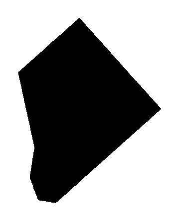
As you can see, Baltimore appears crooked when compared to most maps. This is because Albers is a conic projection so the meridians will not be perpendicular with the top of the SVG element when translating. If we center on latitude and rotate on longitude by making the following change to the projection:

var projection = d3.geo.albers()
    .center([0, 39.3])
    .rotate([76.6, 0])
    ...

This gives an image that is more familiar:

Next, we can add the roads, streams and rivers, and shorelines to our map by adding the following to the d3.json() function:

svg.selectAll(".feature-code")
    .data(edges.features)
    .enter().append("path")
    .attr("d", path)
    .attr("class", function (d) { return "feature-code " + d.properties.code; });

This code selects all child elements of our SVG element with the feature-code class and the data function joins it with the list of edges from our TopoJSON file. The enter function appends a path element to the SVG for every new element encountered. Since the SVG element did not have any children with the feature-code class, a new path is added for each edge. Finally, it adds two classes to each new element: feature-code and the MTFCC code that we mapped to the code property earlier.

Similarly, we can add a label for the map by adding the following to the d3.json() function:

svg.selectAll(".label")
    .data(baltimore.features)
    .enter().append("text")
    .attr("class", "label")
    .attr("transform", function(d) { return "translate(" + path.centroid(d) + ")"; })
    .attr("dy", ".35em")
    .text(function(d) { return d.properties.name; });

The code works similarly. We start with the SVG and select all of its child elements with the label class. We join this with everything from the list of places (which contains only Baltimore) from our combined TopoJSON file.

Without styling, our map is still black. We can change this by adding the following CSS to the style block in the HTML head element:

.label {
    fill: #777;
    fill-opacity: .5;
    font-size: 20px;
    font-weight: 300;
    text-anchor: middle;
}
.baltimore {
    fill: #ffa500;
}
.water {
    fill: #1047a9;
}
.feature-code {
    fill: None;
}
.H3010 {
    stroke: #4577d4;
    stroke-width: 1;
}
.S1100 {
    stroke: #a66c00;
    stroke-width: 2;
}
.P0002, .P0003 {
    stroke: #bf8d30;
    stroke-width: 1;
}

After styling, our map looks like this:

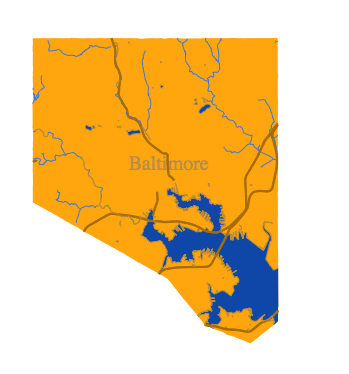
There you have it! Our final HTML should look like:

<!DOCTYPE html>
<html>
<head>
<meta charset="utf-8">
<style>

.label {
    fill: #777;
    fill-opacity: .5;
    font-size: 20px;
    font-weight: 300;
    text-anchor: middle;
}
.baltimore {
    fill: #ffa500;
}
.water {
    fill: #1047a9;
}
.feature-code {
    fill: None;
}
.H3010 {
    stroke: #4577d4;
    stroke-width: 1;
}
.S1100 {
    stroke: #a66c00;
    stroke-width: 2;
}
.P0002, .P0003 {
    stroke: #bf8d30;
    stroke-width: 1;
}
</style>
<style type="text/css"></style></head><body>
<script src="http://d3js.org/d3.v3.min.js"></script>
<script src="http://d3js.org/topojson.v1.min.js"></script>
<script>
var width = 400,
    height = 400;

var projection = d3.geo.albers()
    .center([0, 39.3])
    .rotate([76.6, 0])
    .parallels([38, 40])
    .scale(100000)
    .translate([width / 2 ,height / 2 ]);

var path = d3.geo.path()
    .projection(projection);

var svg = d3.select("body").append("svg")
    .attr("width", width)
    .attr("height", height);

d3.json("balt.json", function(error, bmore) {
    if (error) return console.log(error);
    var edges = topojson.feature(bmore, bmore.objects.baltimore_edges),
        water = topojson.feature(bmore, bmore.objects.baltimore_water),
        baltimore = topojson.feature(bmore, bmore.objects.baltimore);
    console.log(water);
    svg.append("path")
        .datum(baltimore)
        .attr("d", path)
        .attr("class", "baltimore");

    svg.append("path")
        .datum(water)
        .attr("d", path)
        .attr("class", "water");

    svg.selectAll(".feature-code")
        .data(edges.features)
        .enter().append("path")
        .attr("d", path)
        .attr("class", function (d) { return "feature-code " + d.properties.code; });

    svg.selectAll(".label")
        .data(baltimore.features)
        .enter().append("text")
        .attr("class", "label")
        .attr("transform", function(d) { return "translate(" + path.centroid(d) + ")"; })
        .attr("dy", ".35em")
        .text(function(d) { return d.properties.name; });
})
</script>
</body>
</html>